ZEDprofiler Walkthrough
ZEDprofiler is a CPU-first toolkit for extracting morphological features from 3D fluorescence microscopy images. It is designed for high-content and high-throughput workflows where images are volumetric z-stacks with multiple spectral channels and segmentation labels.
What this walkthrough covers
By the end of this notebook you will have:
Generated synthetic 3D image data: two channels (a compact nuclear stain and a diffuse marker with per-object colocalization) and a ground-truth label mask
Explored the data interactively: browsed the z-stack volume with a slice-by-slice viewer
Loaded image sets and objects: configured
ImageSetLoader,ObjectLoader, andTwoObjectLoaderto feed data into the pipelineExtracted six feature classes: colocalization, granularity, intensity, neighbors, texture, and volume/size/shape
Merged all features into a single profile DataFrame with one row per object, following the ZEDprofiler naming convention
Normalized and feature selected the profile using
Pycytominer: z-scoring features and removing low-variance and redundant columnsVisualized pairwise object similarity: computed and plotted a Pearson correlation heatmap across all objects
Each section includes a brief description of what is being computed and what the key parameters control.
Imports
import logging
import warnings

# suppress third-party noise before any imports
logging.basicConfig(level=logging.WARNING)
logging.getLogger("matplotlib").setLevel(logging.WARNING)
warnings.filterwarnings("ignore", category=SyntaxWarning, module="mahotas")

import pathlib

import numpy as np
import pandas as pd
import tifffile
from itables import show

import zedprofiler
from zedprofiler.IO import loading_classes
annotation=NoneType required=False default_factory=list
/home/docs/checkouts/readthedocs.org/user_builds/zedprofiler/envs/latest/lib/python3.13/site-packages/mahotas/morph.py:322: SyntaxWarning: invalid escape sequence '\s'
  with ``1``\s, while the ``0``\s line up with ``0``\s (``2``\s correspond to
/home/docs/checkouts/readthedocs.org/user_builds/zedprofiler/envs/latest/lib/python3.13/site-packages/mahotas/features/texture.py:111: SyntaxWarning: invalid escape sequence '\|'
  Feature 10 (index 9) has two interpretations, as the variance of \|x-y\|
/home/docs/checkouts/readthedocs.org/user_builds/zedprofiler/envs/latest/lib/python3.13/site-packages/mahotas/features/texture.py:223: SyntaxWarning: invalid escape sequence '\|'
  Feature 10 (index 9) has two interpretations, as the variance of \|x-y\|
Define Paths and Parameters
This walkthrough uses synthetically generated 3D arrays so it runs anywhere without real microscopy data. Two random intensity channels and a label mask are generated from spherical objects placed at known positions.
The channel_mapping dictionary maps logical names to substrings found in your image filenames: ZEDprofiler uses these keys to identify which file corresponds to which channel or segmentation label.
Expand the cells below to see how paths are configured and how the synthetic data is generated.
Generated volume: (80, 80, 30), objects: 6
Channel 1: nuclear stain (compact)
Channel 2: diffuse stain (per-object colocalization strength varies)
Preview Synthetic Data
The interactive viewer below shows a z-slice browser for all three arrays. Use the slider to step through the volume and see how the objects and their labels change across z-planes.
Expand the cell below to see how the interactive viewer is built.
Loading Objects and Image Sets
ZEDprofiler uses three loader classes to organize image data before featurization:
ImageSetConfig: declares which keys are raw intensity channels (raw_image_key_name) and which are segmentation labels (label_key_name). This config is passed to the loader so it knows how to partition the channel mapping.ImageSetLoader: loads the full image set from disk (or from in-memory arrays) and stores each channel and label as a numpy array. Theanisotropy_spacingparameter describes the physical voxel size in[z, y, x]order and is used by downstream features (e.g. neighbors, surface area) that require real-world distances.ObjectLoader: a lightweight view over one channel + one compartment within a loaded image set. Most featurization functions accept anObjectLoader.TwoObjectLoader: a paired view over two channels within one compartment, required by colocalization which compares signal across two channels simultaneously.
isc = loading_classes.ImageSetConfig(
    image_set_name="test_image_set",
    raw_image_key_name=[CHANNEL1, CHANNEL2],
    label_key_name=[COMPARTMENT],
)

image_set_loader = loading_classes.ImageSetLoader(
    anisotropy_spacing=[1, 0.1, 0.1],
    channel_mapping=channel_mapping,
    image_set_path=image_set_path,
    label_set_path=label_set_path,
    config=isc,
    # we can also directly pass arrays.
    # This is what ZEDprofiler expects when the images are multichannel.
    # Load the image arrays in and pass them in directly instead
    # of loading from path.
    image_set_array=None,
    label_set_array=None,
)
ol = loading_classes.ObjectLoader(
    image_set_loader=image_set_loader,
    channel_name=CHANNEL1,
    compartment_name=COMPARTMENT,
)
coloc_loader = loading_classes.TwoObjectLoader(
    image_set_loader=image_set_loader,
    compartment=COMPARTMENT,
    channel1=CHANNEL1,
    channel2=CHANNEL2,
)
Colocalization
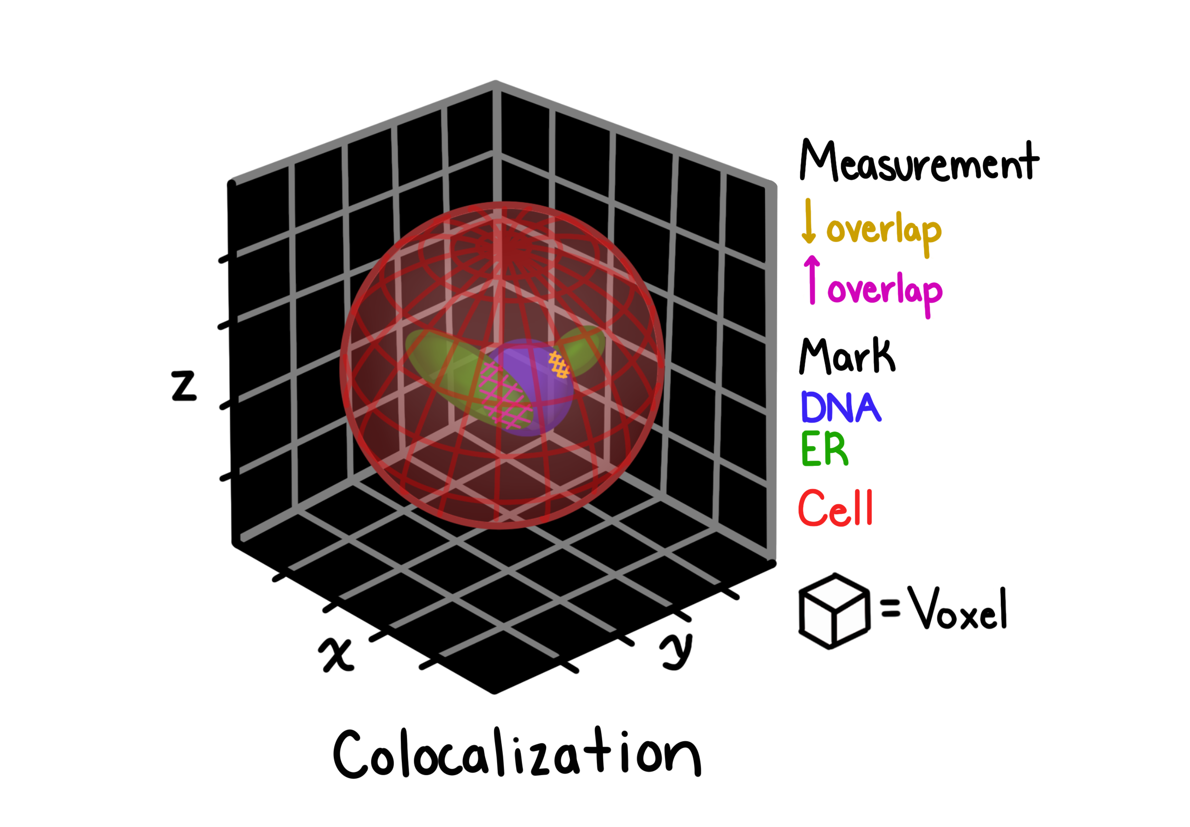
Colocalization measures the degree to which two fluorescent channels occupy the same spatial locations within a segmented compartment. This is useful for quantifying co-expression or co-localization of proteins in 3D cell images.
ZEDprofiler computes several colocalization coefficients per object pair:
Pearson correlation: linear correlation of pixel intensities between the two channels
Manders coefficients (M1, M2): fraction of channel 1 (or 2) signal that overlaps with channel 2 (or 1)
Costes thresholded Manders: Manders coefficients computed above a statistically determined threshold
Overlap coefficient: combined spatial and intensity overlap
Rank-weighted colocalization (RWC): robust to intensity differences, weights overlap by rank
Key parameters:
thr: minimum pixel intensity threshold below which pixels are excludedfast_costes:"Accurate"uses the full bisection algorithm for the Costes threshold;"Fast"uses a linear approximation
For full feature definitions, see the Colocalization reference page.
colocalization_features = zedprofiler.colocalization.compute_colocalization(
    two_object_loader=coloc_loader,
    thr=15,
    fast_costes="Accurate",
    channel1=CHANNEL1,
    channel2=CHANNEL2,
)
Granularity
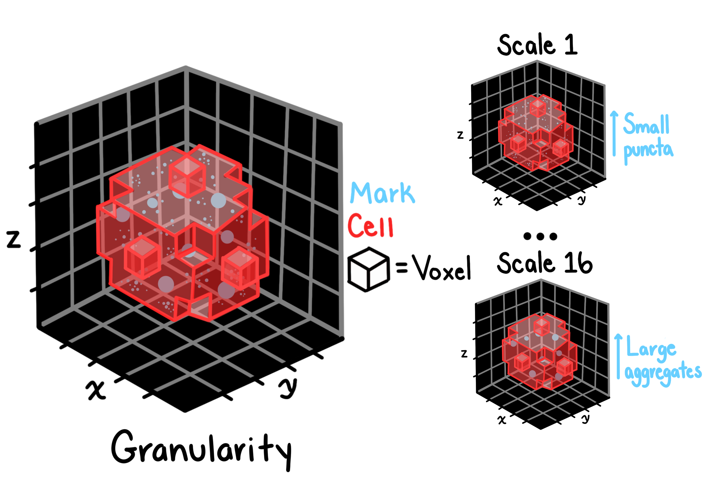
Granularity characterizes the texture of an object at multiple spatial scales by repeatedly applying morphological erosions and measuring how much signal is removed at each scale. The result is a spectrum of values: one per scale: that captures whether an object’s intensity is concentrated in fine, coarse, or mixed-scale structures. This is analogous to CellProfiler’s granularity module and is particularly useful for distinguishing organelle morphology.
Key parameters:
granular_spectrum_length: number of erosion scales to compute (default 16); higher values capture coarser structureradius: radius of the structuring element used for background subtraction before the spectrum is computedsubsample_size: fraction of the image used during spectrum computation (speeds up processing on large volumes)image_sample_size: fraction used for background estimationmask_threshold: threshold applied after interpolation to define the object mask
For full feature definitions, see the Granularity reference page.
granularity_features = zedprofiler.granularity.compute_granularity(
    object_loader=ol,
    radius=10,  # radius of the structuring element for background
    # removal (CellProfiler default)
    granular_spectrum_length=16,  # range of the granular spectrum
    subsample_size=0.25,  # subsample the image for faster processing
    image_sample_size=0.25,  # further subsample for background removal
    mask_threshold=0.9,  # threshold for determining mask after interpolation
    verbose=False,  # print out intermediate steps and values for debugging
)
Intensity
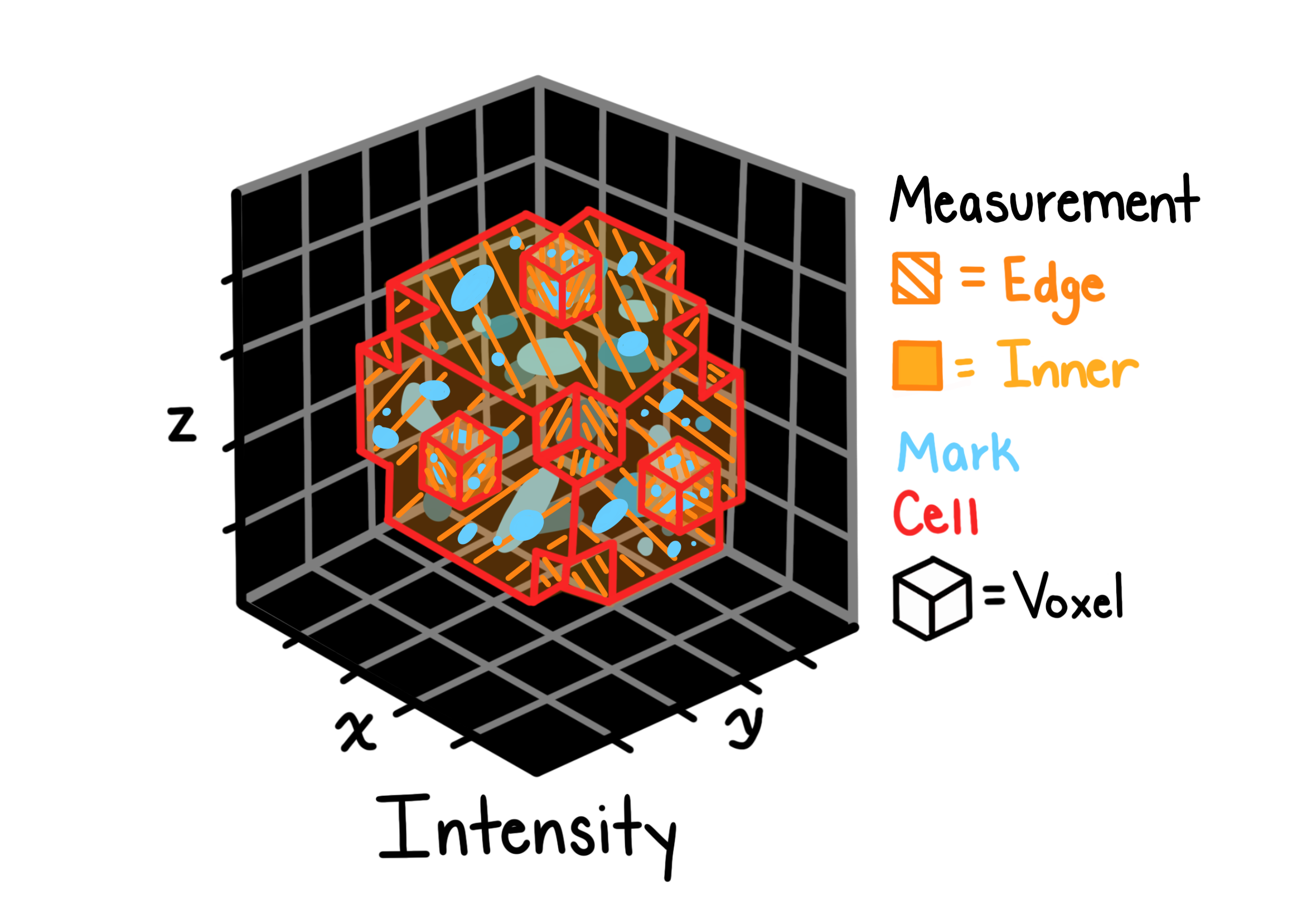
Intensity features summarize the distribution of pixel intensities within each segmented object. They provide a compact description of how bright an object is, how variable its signal is, and how that signal is spatially distributed relative to the object’s edges.
Features computed per object include:
Mean, median, standard deviation, max, min of voxel intensities
Integrated intensity: sum of all voxel intensities (correlated with object volume)
Mass displacement: distance between the object’s geometric centroid and its intensity-weighted centroid, indicating asymmetric signal distribution
Lower/upper quartile intensities: robust measures of the intensity distribution
For full feature definitions, see the Intensity reference page.
intensity_features = zedprofiler.intensity.compute_intensity(
    object_loader=ol,
)
Neighbors
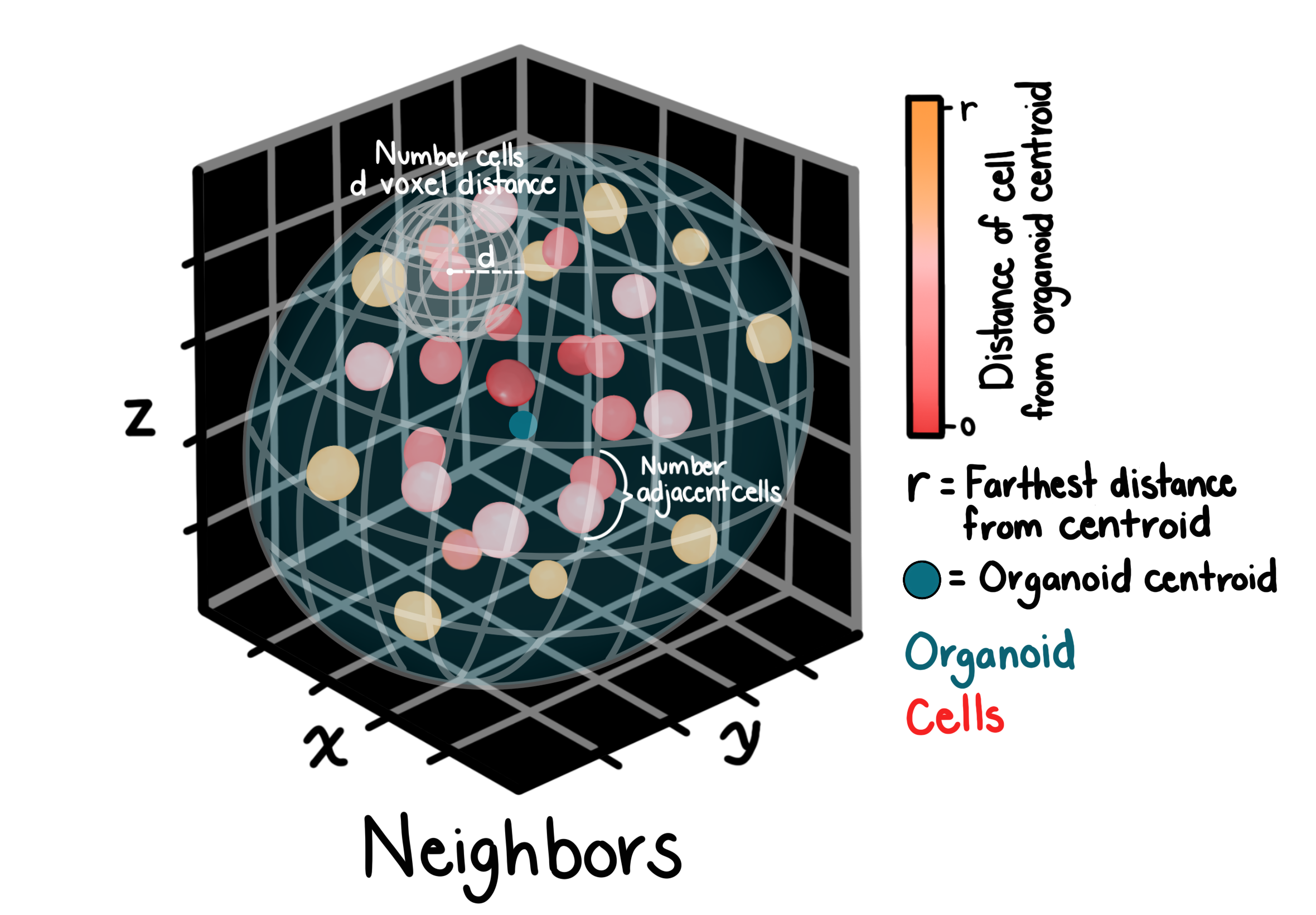
Neighbor features describe the spatial relationships between objects within a compartment. For each object, ZEDprofiler identifies all other objects whose centroids fall within a given distance and computes summary statistics over that neighborhood.
Features include counts of neighbors, mean and standard deviation of distances to neighbors, and the angle between each object and its closest neighbor.
Key parameters:
distance_threshold: maximum centroid-to-centroid distance (in voxels) for two objects to be considered neighborsanisotropy_factor: the ratio of z-spacing to xy-spacing (anisotropy_spacing[0] / anisotropy_spacing[1]); used to rescale z-distances to physical units before computing Euclidean distances, ensuring accurate neighbor relationships in anisotropic volumes
For full feature definitions, see the Neighbors reference page.
neighbors_features = zedprofiler.neighbors.compute_neighbors(
    object_loader=ol,
    distance_threshold=10,
    anisotropy_factor=image_set_loader.anisotropy_spacing[0]
    / image_set_loader.anisotropy_spacing[
        1
    ],  # z to xy spacing ratio for distance calculation
)
Texture
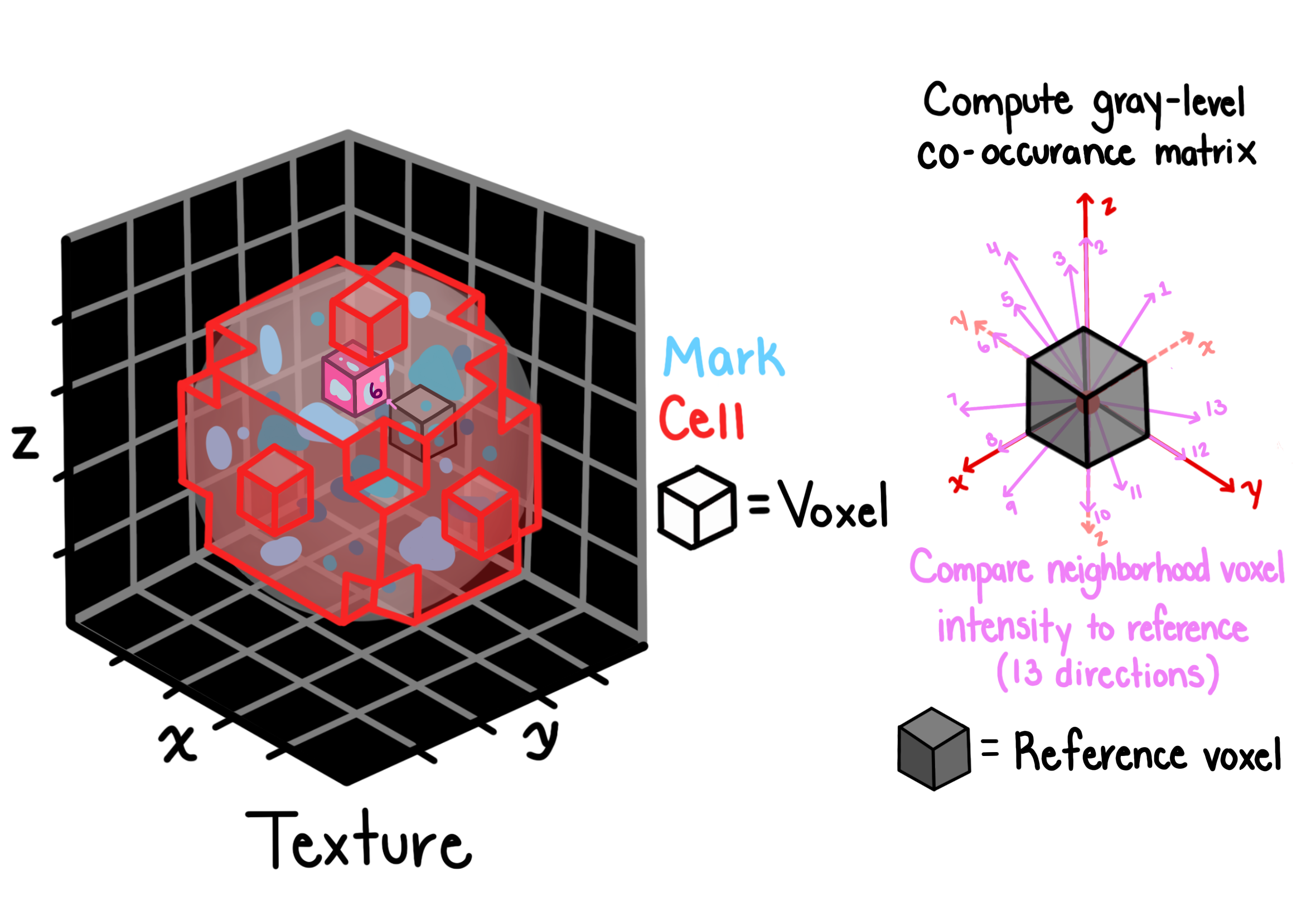
Texture features capture the spatial arrangement of intensities within an object using the gray-level co-occurrence matrix (GLCM). The GLCM records how often pairs of pixel intensities occur at a given spatial offset, and summary statistics computed from it describe properties like smoothness, contrast, and periodicity.
ZEDprofiler computes GLCM-based features (e.g. angular second moment, contrast, correlation, entropy, homogeneity) at multiple offsets and directions in 3D, then aggregates across directions.
Key parameters:
distance: the pixel offset at which co-occurrence is measured; larger values capture coarser texture patternsgrayscale: the number of intensity bins used to quantize the image before computing the GLCM; fewer bins are faster but lose intensity resolution
For full feature definitions, see the Texture reference page.
texture_features = zedprofiler.texture.compute_texture(
    object_loader=ol,
    distance=3,
    grayscale=256,
)
Volume, Size, and Shape
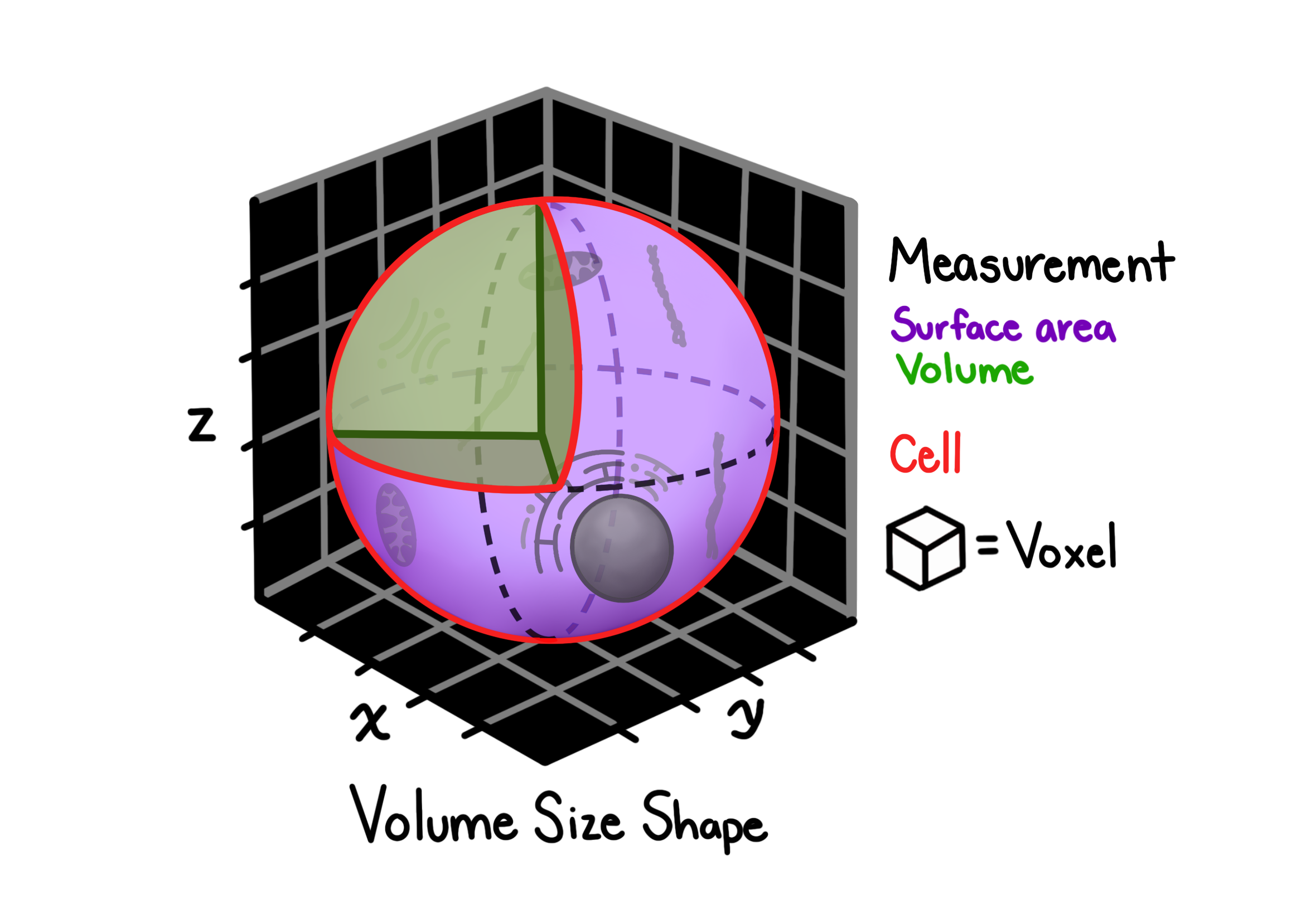
Volume, size, and shape features characterize the 3D geometry of each segmented object.
They are computed using skimage.measure.regionprops on the label image, with surface area calculated via marching cubes.
Features per object include:
Volume: total number of voxels in the object
Bounding box: min/max extents in x, y, z
BboxVolume: volume of the axis-aligned bounding box
Centroid: geometric center in x, y, z
Extent: ratio of object volume to bounding box volume (compactness)
Euler number: topological measure of holes/tunnels in the object
Equivalent diameter: diameter of a sphere with the same volume
Surface area: estimated via marching cubes on the object boundary
For full feature definitions, see the Volume, Size, and Shape reference page.
volume_size_shape_features = zedprofiler.volumesizeshape.compute_volume_size_shape(
    image_set_loader=image_set_loader,
    object_loader=ol,
)
Merging All Features into a Single Profile
Each featurization function returns a dictionary that can be converted to a DataFrame.
All DataFrames share two index columns: Metadata_Experiment_ImageSet and Metadata_Object_ObjectID: which are used as merge keys.
The final merged DataFrame contains one row per object and one column per feature, following the ZEDprofiler naming convention:
{Compartment}_{Channel}_{FeatureType}_{Measurement}
See the Feature Schema for the full specification of how columns are named and structured.
The cell below also estimates the total expected feature count when scaling to a full experiment with multiple compartments and channels, giving a sense of the profile dimensionality at scale.
coloc_df = pd.DataFrame(colocalization_features)
granularity_df = pd.DataFrame(granularity_features)
intensity_df = pd.DataFrame(intensity_features)
neighbors_df = pd.DataFrame(neighbors_features)
texture_df = pd.DataFrame(texture_features)
volume_size_shape_df = pd.DataFrame(volume_size_shape_features)
# subtract 2 from each df shape to account for image_set and object_id
# columns that will be used for merging
size_of_all_dfs = [
    df.shape[1] - 2
    for df in [
        coloc_df,
        granularity_df,
        intensity_df,
        neighbors_df,
        texture_df,
        volume_size_shape_df,
    ]
]
# add the 2 back to account for the image_set and object_id columns
# that will be retained in the final merged DataFrame
expected_num_columns = sum(size_of_all_dfs) + 2
columns_to_merge = ["Metadata_Experiment_ImageSet", "Metadata_Object_ObjectID"]

for df in [
    coloc_df,
    granularity_df,
    intensity_df,
    neighbors_df,
    texture_df,
    volume_size_shape_df,
]:
    if not all(col in df.columns for col in columns_to_merge):
        raise ValueError(
            f"DataFrame is missing required columns for merging: {columns_to_merge}"
        )
# merge all features into a single DataFrame
all_features_df = pd.merge(
    coloc_df,
    pd.merge(
        granularity_df,
        pd.merge(
            intensity_df,
            pd.merge(
                neighbors_df,
                pd.merge(
                    texture_df, volume_size_shape_df, on=columns_to_merge, how="inner"
                ),
                on=columns_to_merge,
                how="inner",
            ),
            on=columns_to_merge,
            how="inner",
        ),
        on=columns_to_merge,
        how="inner",
    ),
    on=columns_to_merge,
    how="inner",
)
if all_features_df.shape[1] != expected_num_columns:
    raise ValueError(
        f"""
        Merged DataFrame has {all_features_df.shape[1]} columns
        but expected {expected_num_columns} based on individual DataFrames"""
    )
print(
    f"Shape: {all_features_df.shape[0]} objects x {all_features_df.shape[1]} features"
)
show(all_features_df)
Shape: 6 objects x 233 features
| Loading ITables v2.8.0 from the internet... (need help?) |
expected_num_compartments = 4
expected_num_of_channels = 4
expected_num_of_total_features = (
    expected_num_columns - 2
)  # subtract 2 for image_set and object_id columns
expected_num_of_total_features = (
    expected_num_of_total_features
    * expected_num_compartments
    * expected_num_of_channels
    + 2
)
expected_num_of_total_features
3698
if all_features_df.shape[1] != expected_num_columns:
    raise ValueError(
        f"Expected {expected_num_columns} columns but got {all_features_df.shape[1]}"
    )
Normalize and Feature Select
With all features merged into a single profile DataFrame, we use Pycytominer to:
Normalize: z-score each feature across objects so all features are on the same scale
Feature select: remove low-variance and highly correlated features that carry redundant information
Pycytominer infers which columns are features (prefixed Nuclei_) and which are metadata (prefixed Metadata_) automatically.
from pycytominer import feature_select, normalize

# z-score normalize across all objects
normalized_df = normalize(
    profiles=all_features_df,
    method="standardize",
    output_file=None,
)

# remove low-variance and highly correlated features
selected_df = feature_select(
    profiles=normalized_df,
    operation=["variance_threshold", "correlation_threshold"],
    output_file=None,
)

meta_cols = [c for c in selected_df.columns if c.startswith("Metadata_")]
feature_cols = [c for c in selected_df.columns if c not in meta_cols]
print(
    f"Features after selection: {len(feature_cols)} (from {all_features_df.shape[1] - len(meta_cols)} original)"
)
Features after selection: 25 (from 231 original)
Pairwise Object Correlation
The heatmap below shows the Pearson correlation between every pair of objects across all selected features. Objects with similar morphological profiles appear as warm (high correlation) clusters; dissimilar objects appear cool.
Each row and column is labelled by object ID.